🏠 Home

Week 4

Data Flow Architecture

Chapter 5

Instructor: Baber Sheikh (Visiting Faculty)

Agenda

  • 5.1 Application domains of DFA
  • 5.2 Benefits and limitations of DFA
  • 5.3 Batch sequential Architecture
  • 5.4 Pipe and filter Architecture

🔄 Week 1 Recap: The Foundation

IEEE Definition

"The fundamental organization of a system embodied in its elements, their relationships to each other and to the environment, and the principles guiding its design and evolution."

🌉 The Bridge Analogy (Crux)

Software Architecture is the bridge between Requirements (What users want) and Implementation (Code we write).

It manages complexity, facilitates communication, and addresses Quality Attributes.

🔄 Week 1 Recap: Quality Attributes

⚠️ The Law of Trade-offs

"You likely cannot maximize all quality attributes simultaneously."

⚙️ Implementation

Maintainability

Testability

Flexibility

Portability

🚀 Runtime

Performance

Security

Availability

Usability

💼 Business

Time to Market

Cost

Lifetime

Target Market

👥 Week 1 Recap: The Stakeholders

💰 Customer vs. 👤 User

Customer: Pays for the system. Defines budget, schedule, and business goals.

User: Actually uses the system. Cares about functionality and usability.

Conflict?

Customer wants "Cheap", User wants "Fast".

🏗️ Architect vs. 💻 Developer

Architect: Strategic designer. Communicates with stakeholders. Ensures Quality Attributes.

Developer: Tactical builder. Focuses on implementation details and algorithms.

Role of Architect: The Bridge between Customer/User needs and Developer implementation.

🔄 Week 2 Crux: Design Space Comparison

Refined definitions for exam preparation.

Perspective Definition & Elements Connectors Properties
Static
(Code / Dev)
Compile-time organization
  • Classes, Files, Packages
Imports, Inheritance, Interfaces Modularity, Maintainability
Runtime
(Execution)
System execution
  • Threads, Processes, Objects
IPC, RPC, Network Calls Performance, Security, Availability
Management
(Teams)
Distribution of work
  • Teams, Roles
Meetings, Docs, Emails Cost, Time-to-market

🔄 Week 2 Recap: Building Blocks

🧱 Components

The core computational units.

  • Processing (Filters)
  • Storage (Databases)
  • Managers (Control)

🔗 Connectors

Interactions between components.

  • Procedure Calls
  • Message Passing
  • Data Access

📋 Constraints

Rules of the system.

  • Protocols
  • Standards
  • Law of Demeter

Architecture = Elements (Components + Connectors) + Constraints + Rationale

🔗 Week 2 Recap: Software Connectors

"Connectors mediate interactions between components."

1. Procedure Call (Synchronous)

The standard function call. Caller waits for Callee.

  • Good for: Data transfer, Computation.
  • Risk: Tight coupling, Blocking.

2. Event (Asynchronous)

Fire and forget. Notifications.

  • Good for: UI inputs, Decoupling systems.
  • Risk: Complex debugging.

3. Data Access

SQL Queries, File I/O. Accessing shared data stores.

4. Stream

Continuous flow of data (e.g., Video, Audio).

🔄 Week 3 Crux: The 4+1 View Model

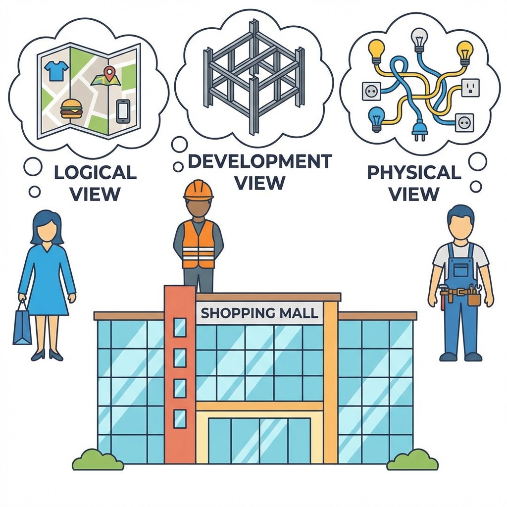
4+1 View Model

⭐ Scenario View (The "+1")

Validates all other views using Use Cases.

Logical

End-user functionality

Process

Runtime / Concurrency

Development

Programmers management

Physical

System Topology

🔄 Week 3 Recap: UML Models

Structure Diagrams (Static)

  • Class Diagram: Static structure of classes.
  • Component Diagram: Physical components.
  • Deployment Diagram: Hardware/Software map.

Behavior Diagrams (Dynamic)

  • Sequence Diagram: Flow of messages over time.
  • Activity Diagram: Workflow logic.
  • State Diagram: State transitions.

🎯 Key Insight

"No single view is sufficient. We need multiple views to describe a system completely."

📝 Week 3 Recap: ADLs

Architecture Description Languages

Why do we need them?

  • Box-and-line diagrams are too informal/ambiguous.
  • Programming code is too detailed.
  • ADLs provide a formal, precise way to document architecture.

Acme ADL Example

System SimpleClientServer = {
  Component client = { Port send; };
  Component server = { Port receive; };
  
  Connector rpc = { 
    Role caller; 
    Role callee; 
  };
  
  Attachment client.send to rpc.caller;
  Attachment server.receive to rpc.callee;
}

Note: UML is a modeling notation, while ADLs are formal languages with strict syntax and semantics for analysis.

Objectives of this Chapter

  • Introduce the concepts of data flow architectures
  • Describe the data flow architecture in UML
  • Discuss the application domains of the data flow architecture approach
  • Assess the benefits and limitations of the data flow architecture approach
  • Demonstrate the batch sequential and pipe and filter architectures in OS and Java scripts

5.1 Overview: Data Flow Architecture

Views the entire software system as a series of transformations on successive sets of data.

🔑 Key Concepts

  • Independence: Data and operations are independent.
  • Decomposition: System is broken into "data processing elements".
  • Control: Data directs and controls the order of computation.

⚙️ Mechanism

Each component transforms its Input Data into corresponding Output Data.

"Data moves from one subsystem to another."

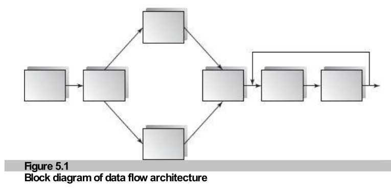
Figure 5.1: Data Flow Block Diagram

Figure 5.1: Block diagram of data flow architecture

(Click to enlarge)

Connections: I/O streams, I/O files, buffers, pipes, etc.

Topology: Graph with cycles, Linear structure, or Tree structure.

Architecture Properties

🧩 Independence (Crux)

No interaction between modules except for input/output data.

Result: High Modifiability & Reusability.

One subsystem can be substituted by another if data format matches.

⚖️ Design Orientation

Can choose either:

  • Traditional Procedure-Oriented
  • Object-Oriented Design

Subsystems do NOT need to know the identity of other subsystems.

Application Domains & Types

Applicable in any domain involving well-defined series of independent data transformations.

✅ Typical Examples

  • Compilers
  • Business Batch Data Processing
  • (Neither require user interaction)

📂 3 Subcategories

  • 1. Batch Sequential
  • 2. Pipe and Filter (Non-sequential pipeline)
  • 3. Process Control (Closed-loop)

5.2 Batch Sequential Architecture

Overview

Traditional data processing model (1950s-1970s). Common in RPG and COBOL.
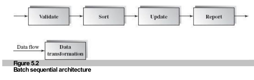
  • Constraint: Subsystem cannot start until previous one completes.
  • Data Flow: Carries a "batch" of data as a whole.
  • Linear Flow: Validate ➜ Sort ➜ Update ➜ Report.
Figure 5.2: Batch Sequential Architecture

Figure 5.2: Validation, Sorting, Updating, Reporting

Detailed Example: Banking & Billing

Goal: Validate transactions, sort by primary key (efficiency), update master file.

Process Steps

  1. Validate: Check inserts/deletes/updates.
  2. Sort: Order transactions to match Master File.
  3. Update: Apply changes to Master.
  4. Report: Generate final list.

Note: Intermediate files are transient and can be removed.
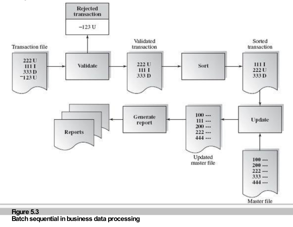
Figure 5.3: Batch Sequential in Business Processing

Implementation: Unix Shell Script

Scripts drive the sequence. Data files are the driving force.

Run: myShell.sh (exec) searching kwd < inputFile> matchedFile (exec) counting < matchedFile> countedFile (exec) sorting < countedFile> myReportFile

Redirect Operators

< : Input from file (stdin)

> : Output to file (stdout)

Substitutability

Can replace executables (e.g., C program ➔ Java) if input/output formats match.

Implementation: Java Template

public class BatchSequential {

    public static void main() {
        searching(kwd, inputFile, matchedFile);
        counting(matchedFile, countedFile);
        sorting(countedFile, reportFile);
    }

    // Static methods belonging to the class, not objects
    public static void searching(String kwd, String in, String out) { ... }
    public static void counting(String in, String out) { ... }
    public static void sorting(String in, String out) { ... }
}
Note: No single instance (Object) is created. Static methods represent the independent processing steps.

Summary: Batch Sequential

📂 Applicable Domains

  • Batched data sets
  • Sequential access files
  • Independent Read/Write steps

✅ Benefits

  • Simple division of tasks
  • Stand-alone programs
  • Easy to valid/test individually

⚠️ Limitations

  • Requires external control (Script)
  • No interactive interface
  • High Latency: No concurrency capability

5.3 Pipe and Filter Architecture

Definition: Decomposes the system into functional components (Filters) connected by data streams (Pipes).

Key Components

  • Filter: Independent data transformer. Local incremental mode.
  • Pipe: Moves data stream. First-In/First-Out buffer.
  • Source/Sink: Origin and destination of data.

Attributes

  • Concurrent: Filters work simultaneously.
  • Incremental: Processing starts as soon as data arrives (no waiting for full batch).
  • Data Stream: Bytes, characters, XML records.

Transmission Modes (Data Flow)

➜ Push Only

Write Only

Data Source or Filter pushes data downstream.

➜ Pull Only

Read Only

Data Sink or Filter pulls data from upstream.

⇄ Pull/Push

Read/Write

Filter pulls data from upstream and pushes transformed data downstream.

Serialization: Object-type data must be serialized to pass through binary/char pipes.

Active vs. Passive Filters

💡 Easy Analogy: Water Pump vs. Funnel

  • Active Filter (Pump): It pulls water in and pushes it out forcefully. It does the work.
  • Passive Filter (Funnel): It just sits there. Water is pushed into it and pulled out by gravity/pipes.
  • Active Filter: "I will go get data, process it, and send it away."
  • Passive Filter: "I will wait for data to be given to me."

Figure 5.4 shows Active Filters connecting to Passive Pipes.
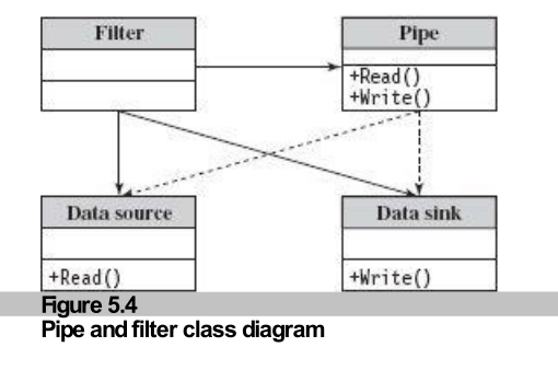
Figure 5.4: Pipe and Filter Class Diagram

Sequence & Pipelining

💡 Easy Analogy: Car Assembly Line

Worker A puts on the tires. Worker B installs the engine. Worker B doesn't wait for Worker A to finish all the cars. As soon as one car is ready, Worker B starts. They work at the same time!

How it flows (Fig 5.5)

Source ➜ Filter 1 ➜ Pipe ➜ Filter 2 ➜ Sink
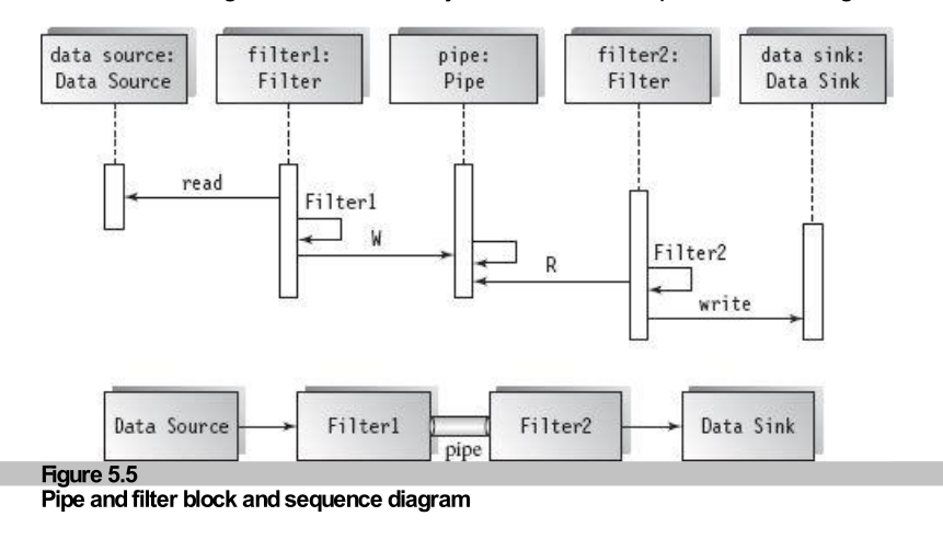
Figure 5.5: Sequence Diagram

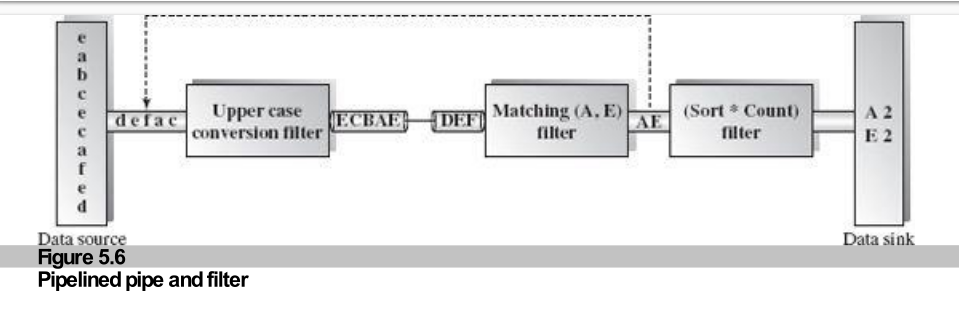
Real Example (Fig 5.6)

Lowercase ➔ Uppercase ➔ Match 'A'

Figure 5.6: Pipelined Example

Blocking vs. Non-Blocking Read

💡 Easy Analogy: Empty Plate at Dinner

  • Blocking (Wait): Your plate is empty. You stop eating and wait until Mom puts more food on it. You can't do anything else.
  • Non-Blocking (Check): You look at the plate. Empty? Okay, you play with your phone instead. You don't freeze.

Blocking Read (Standard): The program halts at read() until data arrives.

Non-Blocking: Returns null or 0 immediately if empty.
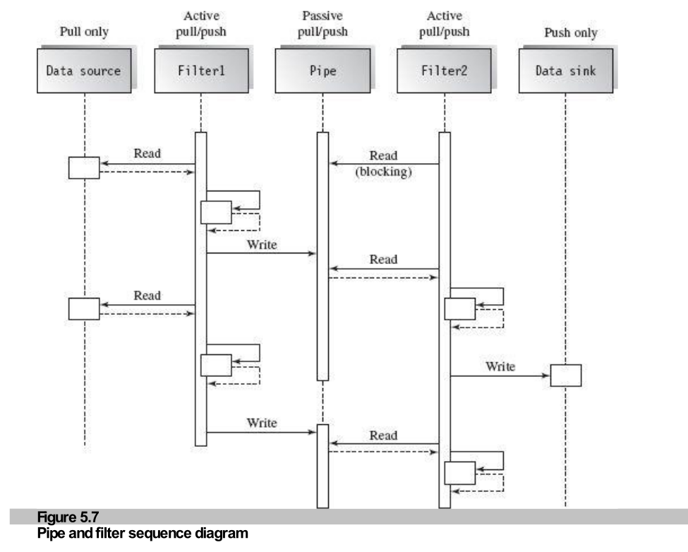
Figure 5.7: Blocking Read Sequence

Unix Implementation: The Pipe |

💡 Easy Example: Counting Online Users

Command: who | wc -l

  1. who: Lists everyone logged in. (Producer)
  2. |: The Pipe (Passes the list).
  3. wc -l: Counts the lines. (Consumer)

They run together! The counter starts counting before the list follows finished.

Named Pipes (Advanced)

Sometimes we need a pipe that stays forever, like a file. That is a Named Pipe (mkfifo).
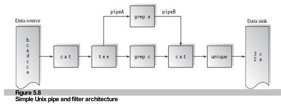
Figure 5.8: Unix Pipe Architecture

Java Implementation

Concept: Two separate Threads (Programs) running at the same time.

Thread A writes to the pipe. Thread B reads from it.

// WAITER (Filter 1): Puts numbers on the tray
public class Filter1 extends Thread {
    PipedWriter pw;
    public void run() {
        for (int j = 1; j < 100; j++) {
            pw.write(j); // Putting data in pipe
        }
    }
}

// CHEF (Filter 2): Takes numbers off the tray
public class Filter2 extends Thread {
    PipedReader pr;
    public void run() {
        while (pr.read() != -1) { 
            // Processing data from pipe
        }
    }
}

Summary: Pipe & Filter

📂 Where to use?

  • When you have steps (A -> B -> C).
  • Multimedia (Video -> Decode -> Display).
  • Compilers (Source -> Lexer -> Parser).

✅ Why is it good?

  • Fast: Everyone works at once (Concurrency).
  • Easy: Just snap blocks together (Plug & Play).

⚠️ What's the catch?

  • Interactive? No. Can't really "talk back" to the user easily.
  • Parsing: Every filter has to read/parse data again.

5.4 Process Control Architecture

💡 Easy Analogy: Cruise Control in a Car

You set the speed to 60mph (Goal). The car checks the speedometer (Sensor). If it's 55mph, it presses the gas (Action). If 65mph, it eases off. It keeps checking and adjusting forever.

Definition: Architecture for embedded systems that maintain a variable (e.g., Temperature, Speed) at a specific level.
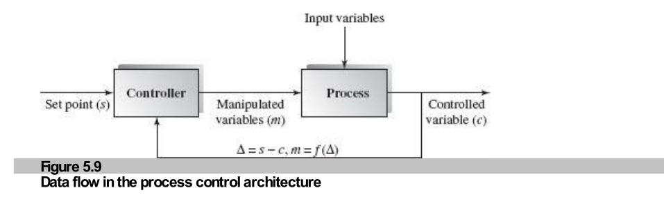
  • Closed Loop: Feedback is used to adjust actions.
  • Decomposition: Whole system = Subsystems + Connections.
Figure 5.9: Process Control Data Flow

Figure 5.9: Feedback Logic

Process Control Variables

A process control system relies on these key data types:

Variable Type Description Example (AC System)
Controlled Variable The target value the system must maintain. Room Temperature
Set Point The goal value defined by the user. 72°F (Thermostat Setting)
Input Variable Measured data from sensors. 78°F (Current Temp)
Manipulated Variable What is adjusted to change the result. Cold Air Flow / Fan Speed

Feedback Loop Logic

Two Main Units

🧠 Controller Unit

The Brain

Calculates the difference:

Error = Set Point - Current Value

Decides how much to adjust.

💪 Executor Unit

The Muscle

Physically changes the process control variables (e.g., Engine, Heater, Motor).

graph LR User[User Set Point] --> Controller Sensor[Sensor Input] --> Controller Controller --Commands--> Executor Executor --Action--> Environment Environment --Feedback--> Sensor

Real World Examples

🚗 Cruise Control

  • Set Point: 60 MPH.
  • Sensor: Wheel Speed.
  • Controller: Computer.
  • Executor: Throttle/Engine.
  • Action: Maintaining speed despite hills/wind.

❄️ AC / HVAC System

  • Set Point: 22°C.
  • Sensor: Thermometer.
  • Controller: Thermostat Logic.
  • Executor: Compressor/Fan.
  • Action: Cooling the air until 22°C is reached.

Domains & Benefits

📂 Applicable Domains

  • Embedded Software: Systems inside devices (Cars, Microwaves, Robots).
  • Continuous Action: Systems that run forever, not start-stop.
  • Stable Output: Systems needing to hold a specific state.

✅ Benefits

  • Precise Control: Better than simple formulas for complex physical environments.
  • Embedded Ready: Logic is completely contained in the device.
  • Responsiveness: Reacts immediately to environmental changes.

5.5 Chapter Summary

Data Flow Architecture decomposes systems into transformation steps connected by data links.

1. Batch Sequential

Step-by-step.

Each step completes fully before the next starts.

Example: Month-end billing.

2. Pipe & Filter

Concurrent Streaming.

Steps run in parallel. Data flows constantly.

Example: Unix Command Line.

3. Process Control

Continuous Feedback.

Maintains a state using loops.

Example: Cruise Control.

Architecture Comparison

Feature Batch Sequential Pipe & Filter Process Control
Data Flow Discrete Batches Continuous Streams Variable Updates
Control Explicit (Step A then B) Implicit (Driven by Data) Loop (Driven by Sensors)
Concurrency None (Sequential) High (Parallel) Real-time
Best For Tape/File Processing Media/Text Streams Embedded Systems

Design Guidelines

💡 How to design a Data Flow System?

Follow these 4 golden rules:

  1. Decompose: Break system into a series of process steps.
  2. Define Formats: Clearly define Input and Output data for each step.
  3. Define Logic: Specify exactly what transformation happens in each step.
  4. Design Pipelines: Use buffering/pipelining if you need speed (concurrency).

Chapter 5 Crux: The Core Takeaways

1. It's All About Movement

Data Flow architecture is not about objects or functions. It's about Movement.

  • How does data get from point A to point B?
  • Does it move in large chunks (Batch) or small streams (Pipe)?

2. The 3 Flavors

  • Batch Sequential: Safe, Simple, Slow. (Bank Processing)
  • Pipe & Filter: Fast, Concurrent, Modular. (Video Streaming)
  • Process Control: Cyclical, Reactive, Embedded. (Thermostat)

🎓 Crux: Choose Batch for simplicity, Pipes for speed, and Control for physical feedback.

When to choose what?

Use this decision logic for your projects:

Scenario A

"I have a massive file. I need to calculate statistics. Precision is key. Time is not critical."


👉 Use Batch Sequential

Scenario B

"I am building a live video editor. Users apply effects while the video plays."


👉 Use Pipe & Filter

Scenario C

"I am programming a drone to hover at a specific altitude."


👉 Use Process Control

Class Activity: The "Human Pipe"

The Mission

We will simulate a Pipe & Filter system manually.

  1. Filter 1 (Producer): Writes a random word on a sticky note.
  2. Pipe A: Passes the note to Filter 2.
  3. Filter 2 (Transformer): Adds an adjective (e.g., "Fast" -> "Fast Cat").
  4. Pipe B: Passes the note to Filter 3.
  5. Filter 3 (Consumer): Draws a picture of the phrase.

⚠️ Rules

  • No Batching: As soon as Filter 1 finishes a word, pass it! Don't wait for 10 words.
  • Concurrency: Filter 1 should write the 2nd word while Filter 2 is processing the 1st word.
  • Goal: See how many drawings we can finish in 2 minutes!

Thank You!

End of Week 4: Data Flow Architectures

Questions?